Machine learning is a lucrative technology, not because of the hype cycle but due to the logic, understanding, and potential it has in solving problems. Let's start with a basic definition of Machine Learning.

Machine Learning, who are you?

Machine learning is nothing, but the machine is learning rather than explicitly feeding it with a series of instructions. The ML algorithms, nothing but some chunk of codes, would create a model, train it to understand the data, and then predict the outcome by giving input.

It's the same as teaching a kid about animals and fruits by giving him some pictures of fruits and animals. We first train the model ( the kid ) with the data and then try to test him by showing other pictures, and he'll be able to predict when he sees something, if it is an animal or a fruit, when he goes out of the room.

Machine Learning has a lot of algorithms, which are different ways of training a model corresponding to the outcome we are expecting or the problem we are trying to solve. some of the important algos to learn are

1. Linear Regression Algorithm

2. Logistic Regression Algorithm

3. Decision Tree

4. SVM

5. Naïve Bayes

6. KNN

7. K-Means Clustering

8. Random Forest

9. Apriori

10. PCA

Before diving into linear regression algorithm, let us understand the pedagogy to learn/master any algorithm in ML or other AI domains.

The Pedagogy to master any ML algorithm

We need to focus on three things while learning an algorithm

1. Why it is called the way it is called - Understanding why linear regression is called linear regression, decoding its name.

2. Intuition - What the algorithm is doing, visualizing it

3. Maths - The mathematics involved in working, making, and in the logic of an algorithm.

4. Coding - the codes of data preparation, pre-processing, making and training the model, prediction by the model, and the Python libraries used.

   • These are the primary steps: develop the fundamentals of the algorithm. The following steps below are for mastering it.

5. Implementing the algorithm on real-world data (feature engineering)

6. Building an end-to-end product - creating a web app and deploying it on the cloud

7. Documentation of the projects - you can document the project by adding it to GitHub, making a YouTube video explaining it, and publishing it on hashnode. This will also help you to revise.

8. REPEATING THIS ON EVERY ALGORITHM.

Further, you can start applying for jobs when you have a good portfolio. Keeping the learning wave thriving may not necessarily be linear but growing.

The Linear Regression Algorithm

1. DECODING THE NAME :

   • Linear regression shows the linear relationship between the independent variable, i.e., X-axis, and the dependent(output) variable, i.e., Y-axis, called linear regression.

$$y=mx+c$$

this is a basic representation of a line, which is the fundamental example of the linear regression model, where x is an independent variable, and from the slope and intercept, we calculate the y values, obviously making it a dependent variable.

• In Linear Regression, Linear means the linear relationship, and regression indicates a statistical relation between the dependent and independent variables.

1. THE INTUITION :

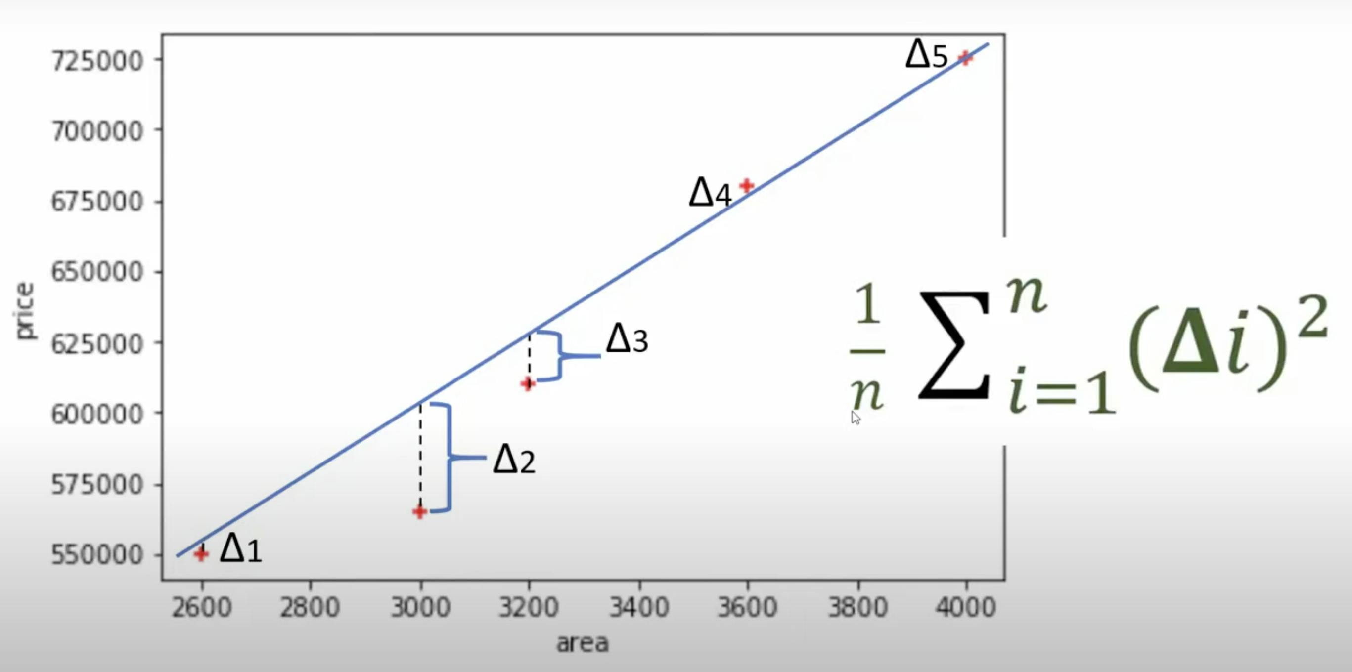
   • Think, you have been given some data points on the XY plane, X indicates the land area, and Y is the price of the land. You are given the task of establishing a relation between these points to predict further prices.

   • The problem would be easier if you had the points that may lie on a line, and we got the line equation, but nature is random. Now, we can try imaging a line that is near all the points or the sum of squares of the distance from points, and the line is minimum.

   • This is what Linear regression does. It finds the best-fit line from the data, establishing the best possible relation between the data points. we then use this line for the prediction of further values (this is how the weather prediction happens; we use more than one feature or independent variable for it )

   • But how do you find that best-fitting line? We'll cover that in the maths section.

• In ML terminology, we call the slope m as 'weight' and intercept c as 'bias.' Below is the general form of an equation. sometimes, the independent variables are called features.

$$y = \beta_0 + \beta_1 x_1 + \beta_2 x_2 +....$$

• y is the dependent variable or the output value.

• x1,x2,x3... are the features.

• beta_1, beta_2... are the weights.

• beta_0 is the bias.

  3. THE MATHEMATICS :

• In the school, we are given a set of X values and a function to find the Y values.

$$\begin{align*} x &= [1, 2, 3, 4, 5] \\ y &= 2x + 4 \\ \\ y &= [6, 8, 12, 14] \end{align*}$$

• But In ML, the reverse happens. We find the equation with the data given.

$$\begin{align*} x &= [1, 2, 3, 4, 5] \\ y &= [6, 8, 12, 14] \\ \\ y &= 2x + 4 \end{align*}$$

Here, we have to find the best-fitting line, as we can draw multiple lines from the given data points. From these, we have to find the best-fitting line. For this, we take a random line from these and calculate the mean of the sum of the squared distance from the line, which is also called Mean Squared Error (MSE) or Cost Function.

$$\begin{align*} MSE = \frac{1}{n} \sum_{i=1}^{n} (y_i - y_{\text{predicted}, i})^2 \\ \\ MSE = \frac{1}{n} \sum_{i=1}^{n} (y_i - mx_i+b )^2 \end{align*}$$

• The gradient descent algorithm helps us find the MSE to find the best-fit line. We are supposed to find the m and b values, i.e., the weights and bias values for which MSE is the least.

• The gradient descent is more like a trial and error where we adjust the values of weights and bias to get the minimum MSE. We take a random m and b value, then decrease them to get the minimum value of MSE.

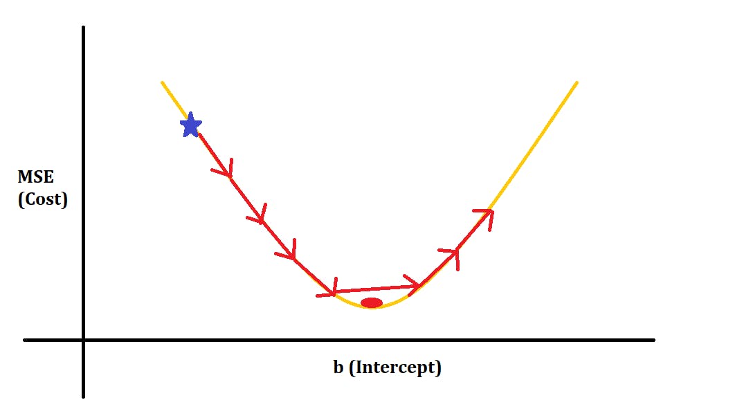
• below is the graph of the cost function concerning the m and b values; for each (m,b), it indicates a line. The point that indicates the minimum of the cost function graph is the one we are trying to find that point indicates the best-fitting line.

• the red ball in the MSE vs. m indicates the slope value corresponding to the best-fitting line

• and the red ball in the MSE vs. b indicates the intercept value corresponding to the best-fitting line.

• But in making this trial and error move, there is a problem. If we take a constant leap of steps in decreasing the m and b values, we may miss the minima some in the mid intervals depicted in the image below.

• 

• to solve this, we take a decreasing rate of lowering m and values in the direction of the curve's tangent to get the m or b values corresponding to the MSE minima.

• 

• we can write them as

$$m = m - \text{{learning rate}} \cdot \frac{{\partial }}{{\partial m}}$$

$$b = b - \text{{learning rate}} \cdot \frac{{\partial }}{{\partial b}}$$

• we can modify the learning rate to get the minimal point, and below is the code for the gradient descent.

•           import numpy as np
  
            def gradient_descent(x,y):
                m_curr = b_curr = 0
                iterations = 10000
                n = len(x)
                learning_rate = 0.08
  
                for i in range(iterations):
                    y_predicted = m_curr * x + b_curr
                    cost = (1/n) * sum([val**2 for val in (y-y_predicted)])
                    md = -(2/n)*sum(x*(y-y_predicted))
                    bd = -(2/n)*sum(y-y_predicted)
                    m_curr = m_curr - learning_rate * md
                    b_curr = b_curr - learning_rate * bd
                    print ("m {}, b {}, cost {} iteration {}".format(m_curr,b_curr,cost, i))
  
            x = np.array([1,2,3,4,5])
            y = np.array([5,7,9,11,13])
  
            gradient_descent(x,y)
  

• when running this code, you will get the cost value by modifying the learning and increasing the number of iterations; after an increased number of iterations, you can see the decrease in the cost value is very minimal and grab the best one as the lower cost, corresponding m and b values to that are the best-fitting line's slope and intercept values.

  1. THE CODE

• we have used sklearn, numpy and pandas libraries to create a linear regression model

• Scikit-learn (sklearn) is a Python library for machine learning that provides simple and efficient data analysis and modelling tools, including various algorithms and utilities for classification, regression, clustering, and dimensionality reduction tasks.

• NumPy: Essential for numerical operations with powerful support for arrays and matrices in Python.

• Pandas: Key library for data manipulation and analysis, leveraging DataFrame structures for efficient data handling and cleaning in Python.

• matplotlib for data visualization. please read the comments to understand the code.

    import numpy as np
    import pandas as pd
    import matplotlib.pyplot as plt
    from sklearn import linear_model
  
    # importing the modules
  

    df = pd.read_csv('house-prices.csv')
    new_df=df.drop('Price',axis='columns')
    new_df
  
    # importing the data
    # droping the price column for the further analysis
  

    # Data Visualization to understadnd the data
  
    x = df.Price #Random x-coordinates
    y = df.SqFt # Random y-coordinates
  
    # Create a scatter plot
    plt.scatter(x, y, label='Scatter Plot', color='blue', marker='o')
  
    # Add labels and a title
    plt.xlabel('X-axis')
    plt.ylabel('Y-axis')
    plt.title('Simple Scatter Plot for home and prices')
  

  
    model = linear_model.LinearRegression() # here, we are creating the model with the linear_model module's LinearRegression() of sklearn library. 
    model.fit(new_df,df.Price) # model training
    prediction = model.predict([[3300],[9000]]) # model prediction with the input values.
    print(prediction)
  

The Wrap Up

This is the complete understanding of the Linear Regression model from scratch. You can do some of the projects on it to understand it more.

Please find the Source Code for the codes.

Stay tuned for more blogs on the projects and other algorithms.